Importing list-of-lists choice data and discrete choice modeling with echoice2
Source:vignettes/Importing_lol_data.Rmd
Importing_lol_data.RmdBackground
Many users have organized their choice data in a list-of-lists
format, where a list of length “number of respondents” is
created, and each element of that lists contains another list with
design matrix and choice information. An example of this is the
camera dataset in ‘bayesm’. echoice2 contains some helper
functions that make it easy to import such data, and estimate
corresponding discrete choice models.
Installation
The echoice2 package is available from CRAN and GitHub.
To install from CRAN, run:
install.packages("echoice2")To install the latest development version from GitHub run:
remotes::install_github("ninohardt/echoice2")Getting started
Load the package.
Key functions for using the package are:
-
vd_est_vdm: Estimating the “standard” volumetric demand model -
vd_est_vdm_screen: Estimating volumetric demand model with screening -
vd_dem_vdm: Demend predictions for the “standard” volumetric demand model -
vd_dem_vdm_screen: Demend predictions for the volumetric demand model with screening
Functions that relate to discrete demand start in dd_,
while functions for volumetric demand start in vd_.
Estimation functions continue in est, demand simulators in
dem. Universal functions (discrete and volumetric choice)
start in ec_.
Data organization
Choice data should be provided in a ‘long’ format tibble or data.frame, i.e. one row per alternative, choice task and respondent.
It should contain the following columns
-
id(integer; respondent identifier) -
task(integer; task number) -
alt(integer; alternative #no within task) -
x(double; quantity purchased) -
p(double; price) - attributes defining the choice alternatives (factor, ordered) and/or
- continuous attributes defining the choice alternatives (numeric)
By default, it is assumed that respondents were able to choose the ‘outside good’, i.e. there is a ‘no-choice’ option. The no-choice option should not be explicitly stated, i.e. there is no “no-choice-level” in any of the attributes. This differs common practice in discrete choice modeling, however, the implicit outside good is consistent with both volumetric and discrete choice models based on economic assumptions.
Dummy-coding is performed automatically to ensure consistency between
estimation and prediction, and to set up screening models in a
consistent manner. Categorical attributes should therefore be provided
as factor or ordered, and not be
dummy-coded.
Importing list-of-list data
Let’s consider the camera example dataset from bayesm.
  library(bayesm)
  data(camera)
  head(camera[[1]]$X)
#>   canon sony nikon panasonic pixels zoom video swivel wifi price
#> 1     0    0     1         0      0    1     0      1    0  0.79
#> 2     1    0     0         0      1    1     0      1    1  2.29
#> 3     0    0     0         1      0    0     0      0    1  1.29
#> 4     0    1     0         0      0    1     0      1    0  2.79
#> 5     0    0     0         0      0    0     0      0    0  0.00
#> 6     0    0     0         1      1    0     0      1    0  2.79
  head(camera[[1]]$y)
#> [1] 1 2 2 4 2 2
Now let’s prepare this dataset for analysis with ‘echoice2’. Using
ec_lol_tidy1 we can stack information from all respondents.
The price variable is renamed to p.
  data_tidier <- ec_lol_tidy1(camera) %>% rename(`p`='price')
  data_tidier %>% head
#> # A tibble: 6 × 14
#>   id     task   alt canon  sony nikon panasonic pixels  zoom video swivel  wifi     p     x
#>   <chr> <int> <int> <dbl> <dbl> <dbl>     <dbl>  <dbl> <dbl> <dbl>  <dbl> <dbl> <dbl> <dbl>
#> 1 1         1     1     0     0     1         0      0     1     0      1     0  0.79     1
#> 2 1         1     2     1     0     0         0      1     1     0      1     1  2.29     0
#> 3 1         1     3     0     0     0         1      0     0     0      0     1  1.29     0
#> 4 1         1     4     0     1     0         0      0     1     0      1     0  2.79     0
#> 5 1         1     5     0     0     0         0      0     0     0      0     0  0        0
#> 6 1         2     1     0     0     0         1      1     0     0      1     0  2.79     0
Looking into the p column, we can see that the 5th
alternative in each task has a price of 0. This is an
explicit outside good which needs to be removed:
  data_tidier_2 <- data_tidier %>% filter(p>0)
  data_tidier_2 %>% head
#> # A tibble: 6 × 14
#>   id     task   alt canon  sony nikon panasonic pixels  zoom video swivel  wifi     p     x
#>   <chr> <int> <int> <dbl> <dbl> <dbl>     <dbl>  <dbl> <dbl> <dbl>  <dbl> <dbl> <dbl> <dbl>
#> 1 1         1     1     0     0     1         0      0     1     0      1     0  0.79     1
#> 2 1         1     2     1     0     0         0      1     1     0      1     1  2.29     0
#> 3 1         1     3     0     0     0         1      0     0     0      0     1  1.29     0
#> 4 1         1     4     0     1     0         0      0     1     0      1     0  2.79     0
#> 5 1         2     1     0     0     0         1      1     0     0      1     0  2.79     0
#> 6 1         2     2     1     0     0         0      1     0     1      0     1  0.79     1
We can already see a couple of brand dummies, which need to be “un-dummied” into a categorical variable. Let’s first check if there are more attributes in dummy form by checking mutually exlusive attributes:
  data_tidier_2 %>% ec_util_dummy_mutualeclusive() %>% filter(mut_ex)
#> # A tibble: 6 × 3
#>   V1    V2        mut_ex
#>   <chr> <chr>     <lgl>
#> 1 canon sony      TRUE
#> 2 canon nikon     TRUE
#> 3 canon panasonic TRUE
#> 4 sony  nikon     TRUE
#> 5 sony  panasonic TRUE
#> 6 nikon panasonic TRUE
As we can see, only brand names come up. “Un-dummying” it is easy
using the ec_undummy function. It has to be supplied with
the column names of the dummies to be un-dummied, and the name of the
target variable, in this case “brand”.
  data_tidier_3 <-
    data_tidier_2 %>% ec_undummy(c('canon','sony','nikon','panasonic'), 'brand')
  data_tidier_3 %>% head
#> # A tibble: 6 × 11
#>   id     task   alt brand     pixels  zoom video swivel  wifi     p     x
#>   <chr> <int> <int> <fct>      <dbl> <dbl> <dbl>  <dbl> <dbl> <dbl> <dbl>
#> 1 1         1     1 nikon          0     1     0      1     0  0.79     1
#> 2 1         1     2 canon          1     1     0      1     1  2.29     0
#> 3 1         1     3 panasonic      0     0     0      0     1  1.29     0
#> 4 1         1     4 sony           0     1     0      1     0  2.79     0
#> 5 1         2     1 panasonic      1     0     0      1     0  2.79     0
#> 6 1         2     2 canon          1     0     1      0     1  0.79     1
The remaining dummies are either high-low or yes-no type binary
attributes. The two utility functions ec_undummy_lowhigh
and ec_undummy_yesno make it convenient to undummy these as
well:
  data_tidied<-
    data_tidier_3 %>%
      mutate(across(c(pixels,zoom), ec_undummy_lowhigh))%>%
      mutate(across(c(swivel,video,wifi), ec_undummy_yesno))
  data_tidied %>% head()
#> # A tibble: 6 × 11
#>   id     task   alt brand     pixels zoom  video swivel wifi      p     x
#>   <chr> <int> <int> <fct>     <fct>  <fct> <fct> <fct>  <fct> <dbl> <dbl>
#> 1 1         1     1 nikon     low    high  no    yes    no     0.79     1
#> 2 1         1     2 canon     high   high  no    yes    yes    2.29     0
#> 3 1         1     3 panasonic low    low   no    no     yes    1.29     0
#> 4 1         1     4 sony      low    high  no    yes    no     2.79     0
#> 5 1         2     1 panasonic high   low   no    yes    no     2.79     0
#> 6 1         2     2 canon     high   low   yes   no     yes    0.79     1
Now data_tidied is ready for analysis.
Checking data
To verify attributes and levels, we can use
ec_summarize_attrlvls:
  data_tidied %>% ec_summarize_attrlvls
#> # A tibble: 6 × 2
#>   attribute levels
#>   <chr>     <chr>
#> 1 brand     canon, nikon, panasonic, sony
#> 2 pixels    low, high
#> 3 zoom      low, high
#> 4 video     no, yes
#> 5 swivel    no, yes
#> 6 wifi      no, yes
Since we have an implicit outside good, let’s check that task total exhibit variation:
  data_tidied %>%
    group_by(id, task) %>%
      summarise(x_total = sum(x), .groups = "keep") %>%
      group_by(x_total) %>% count(x_total)
#> # A tibble: 2 × 2
#> # Groups:   x_total [2]
#>   x_total     n
#>     <dbl> <int>
#> 1       0  1343
#> 2       1  3969
Holdout
For hold-out validation, we keep 1 task per respondent. In v-fold cross-validation, this is done several times. However, each re-run of the model may take a while. For this example, we only use 1 set of holdout tasks. Hold-out evaluations results may vary slightly between publications that discuss this dataset.
  #randomly assign hold-out group, use seed for reproducible plot
  set.seed(555)
    data_ho_tasks=
    data_tidied %>%
      distinct(id,task) %>%
      mutate(id=as.integer(id))%>%
      group_by(id) %>%
      summarise(task=sample(task,1), .groups = "keep")
  set.seed(NULL)

  #calibration data
    data_cal= data_tidied %>% mutate(id=as.integer(id)) %>%
      anti_join(data_ho_tasks, by=c('id','task'))

  #'hold-out' data
    data_ho= data_tidied %>% mutate(id=as.integer(id)) %>%
      semi_join(data_ho_tasks, by=c('id','task'))
Estimation
Estimate both models using at least 200,000 draws. Saving
each 50th or 100th draw is sufficient. The vd_est_vdm fits
the compensatory volumetric demand model, while
vd_est_vdm_screen fits the model with attribute-based
conjunctive screening. Using the error_dist argument, the
type of error distribution can be specified. While KHKA 2022
assume Normal-distributed errors, here we assume Extreme Value Type 1
errors.
  #compensatory
  out_camera_compensatory <- dd_est_hmnl(data_tidied)
  dir.create("draws")
  save(out_camera_compensatory,file='draws/out_camera_cal.rdata')

  #conjunctive screening
  out_camera_screening <- dd_est_hmnl_screen(data_tidied)
  save(out_camera_screening,file='draws/out_camera_screening.rdata')
Diagnostics
Quick check of convergence, or stationarity of the traceplots.
Compensatory:
out_camera_compensatory %>% ec_trace_MU(burnin = 100)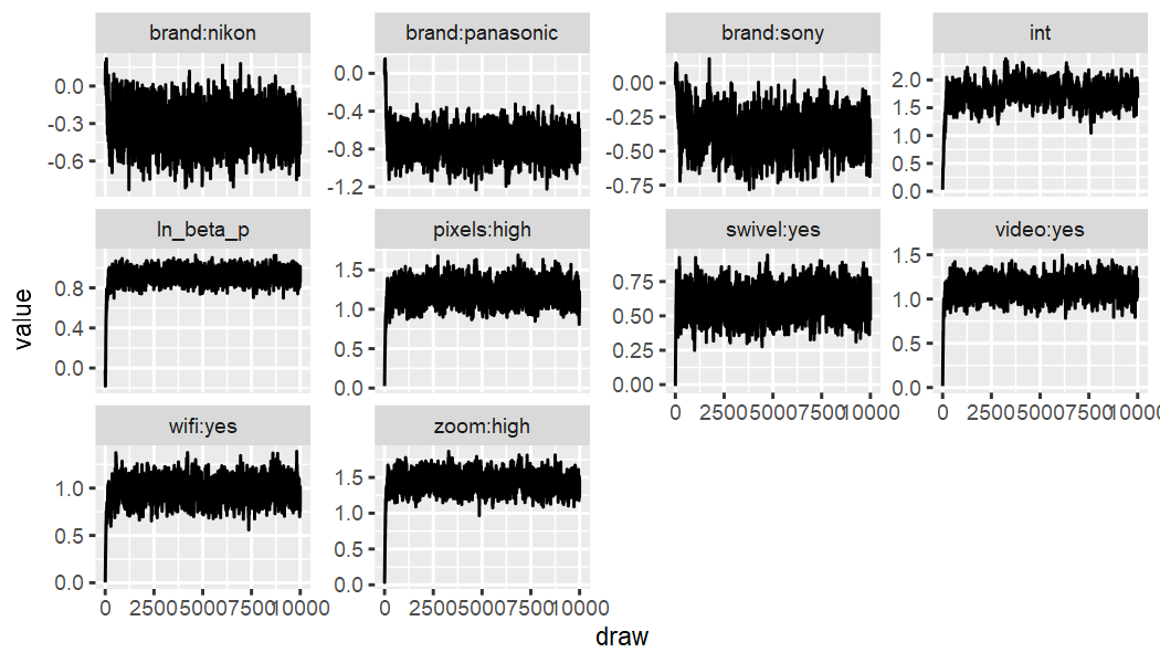
Conjunctive Screening:
out_camera_screening %>% ec_trace_MU(burnin = 100)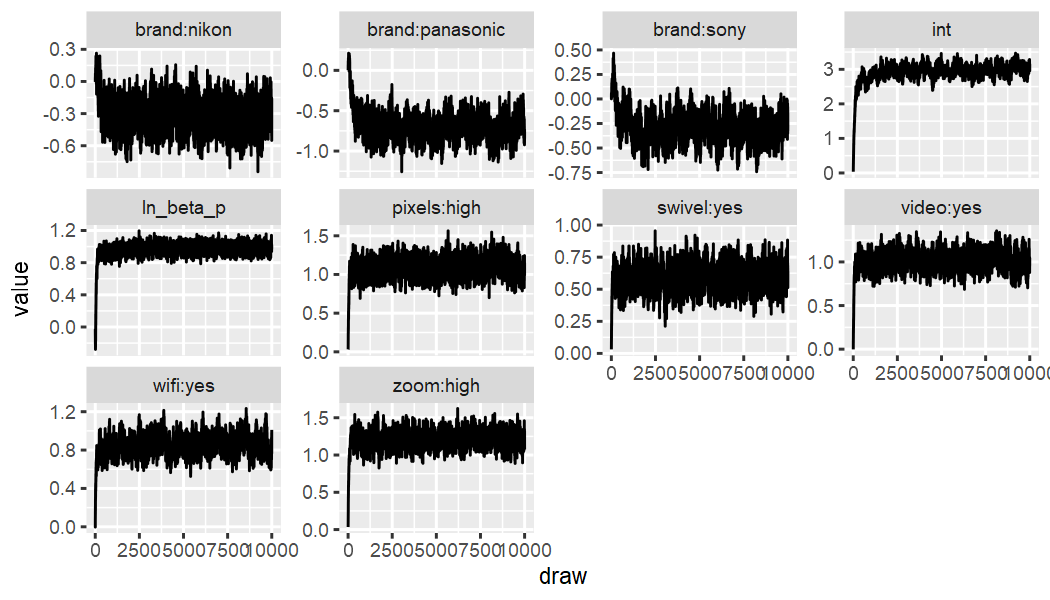
Distribution of Log-likehoods to check for outlier respondents:
  dd_LL(out_camera_compensatory ,data_cal, fromdraw = 3000) %>%
    apply(1,mean) %>% tibble(LL=.) %>%
    ggplot(aes(x=LL)) +
      geom_density(fill="lightgrey", linewidth=1) + theme_minimal() +
      xlab("Individual average Log-Likelihood")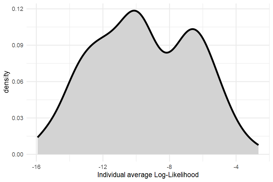
All average log-likelihoods are better than random selection, indicating good data quality.
Fit
Holdout
Now, we compare “holdout”-fit. Here we obtain posterior distributions
of choice share predictions via dd_dem and
dd_dem_sr and then compute the hit probabilities. It is
adviced to carefully think about your relevant loss function and choose
an appropriate metric for holdout fit comparisons.
ho_prob_dd=
    data_ho %>%
      prep_newprediction(data_cal) %>%
        dd_dem(out_camera_compensatory, prob=TRUE)

ho_prob_ddscreen=
    data_ho %>%
      prep_newprediction(data_cal) %>%
        dd_dem_sr(out_camera_screening, prob=TRUE)

hit_probabilities=c()

hit_probabilities$compensatory=
ho_prob_dd %>%
  vd_dem_summarise() %>%
  select(id,task,alt,x,p,`E(demand)`) %>%
  group_by(id,task) %>% group_split() %>%
  purrr::map_dbl(. %>%  select(c(x,`E(demand)`)) %>%
                        add_row(x=1-sum(.$x),`E(demand)`=1-sum(.$`E(demand)`)) %>%
                        summarise(hp=sum(x*`E(demand)`))%>% unlist) %>% mean()

hit_probabilities$screening=
ho_prob_ddscreen %>%
  vd_dem_summarise() %>%
  select(id,task,alt,x,p,`E(demand)`) %>%
  group_by(id,task) %>% group_split() %>%
  purrr::map_dbl(. %>%  select(c(x,`E(demand)`)) %>%
                        add_row(x=1-sum(.$x),`E(demand)`=1-sum(.$`E(demand)`)) %>%
                        summarise(hp=sum(x*`E(demand)`))%>% unlist) %>% mean()

hit_probabilities
#> $compensatory
#> [1] 0.4294928
#>
#> $screening
#> [1] 0.4666976
Estimates
Part-Worths
Using ec_estimates_MU it is easy to obtain the “upper
level” posterior means of the key parameters. We can see that Canon is
the most popular brand. All brand “part-worths” are larger when
accounting for screening, but it is particularly noticeable for Sony and
Panasonic.
  out_camera_compensatory %>% ec_estimates_MU()
#> # A tibble: 10 × 12
#>    attribute lvl       par               mean     sd `CI-5%` `CI-95%` sig   model     error reference_lvl parameter
#>    <chr>     <chr>     <chr>            <dbl>  <dbl>   <dbl>    <dbl> <lgl> <chr>     <chr> <chr>         <chr>
#>  1 brand     nikon     brand:nikon     -0.322 0.134   -0.538   -0.103 TRUE  hmnl-comp EV1   canon         nikon
#>  2 brand     panasonic brand:panasonic -0.736 0.139   -0.945   -0.527 TRUE  hmnl-comp EV1   canon         panasonic
#>  3 brand     sony      brand:sony      -0.360 0.126   -0.557   -0.151 TRUE  hmnl-comp EV1   canon         sony
#>  4 pixels    high      pixels:high      1.22  0.128    1.03     1.41  TRUE  hmnl-comp EV1   low           high
#>  5 zoom      high      zoom:high        1.43  0.126    1.25     1.61  TRUE  hmnl-comp EV1   low           high
#>  6 video     yes       video:yes        1.12  0.106    0.958    1.28  TRUE  hmnl-comp EV1   no            yes
#>  7 swivel    yes       swivel:yes       0.597 0.0931   0.448    0.750 TRUE  hmnl-comp EV1   no            yes
#>  8 wifi      yes       wifi:yes         0.980 0.114    0.801    1.16  TRUE  hmnl-comp EV1   no            yes
#>  9 <NA>      <NA>      int              1.74  0.199    1.47     2.02  TRUE  hmnl-comp EV1   <NA>          int
#> 10 <NA>      <NA>      ln_beta_p        0.919 0.0809   0.821    1.01  TRUE  hmnl-comp EV1   <NA>          ln_beta_p
  out_camera_screening %>% ec_estimates_MU()
#> # A tibble: 10 × 12
#>    attribute lvl       par               mean     sd `CI-5%` `CI-95%` sig   model        error reference_lvl parameter
#>    <chr>     <chr>     <chr>            <dbl>  <dbl>   <dbl>    <dbl> <lgl> <chr>        <chr> <chr>         <chr>
#>  1 brand     nikon     brand:nikon     -0.309 0.143   -0.536  -0.0680 TRUE  hmnl-conj-pr EV1   canon         nikon
#>  2 brand     panasonic brand:panasonic -0.687 0.163   -0.920  -0.448  TRUE  hmnl-conj-pr EV1   canon         panasonic
#>  3 brand     sony      brand:sony      -0.284 0.149   -0.509  -0.0405 TRUE  hmnl-conj-pr EV1   canon         sony
#>  4 pixels    high      pixels:high      1.08  0.120    0.904   1.27   TRUE  hmnl-conj-pr EV1   low           high
#>  5 zoom      high      zoom:high        1.21  0.115    1.04    1.38   TRUE  hmnl-conj-pr EV1   low           high
#>  6 video     yes       video:yes        1.01  0.107    0.852   1.18   TRUE  hmnl-conj-pr EV1   no            yes
#>  7 swivel    yes       swivel:yes       0.588 0.0935   0.438   0.740  TRUE  hmnl-conj-pr EV1   no            yes
#>  8 wifi      yes       wifi:yes         0.852 0.104    0.692   1.02   TRUE  hmnl-conj-pr EV1   no            yes
#>  9 <NA>      <NA>      int              2.92  0.263    2.59    3.21   TRUE  hmnl-conj-pr EV1   <NA>          int
#> 10 <NA>      <NA>      ln_beta_p        0.965 0.0899   0.873   1.06   TRUE  hmnl-conj-pr EV1   <NA>          ln_beta_p
Screening probabilities
Using ec_estimates_screen, screening probabilities be
obtained. As we can see, screening does not play a huge role in this
dataset, and therefore improvements in fit are just modest.
  out_camera_screening %>% ec_estimates_screen()
#> # A tibble: 14 × 8
#>    attribute lvl       par                mean     sd  `CI-5%` `CI-95%` limit
#>    <chr>     <chr>     <chr>             <dbl>  <dbl>    <dbl>    <dbl> <dbl>
#>  1 brand     canon     brand:canon     0.0247  0.0489 0.00572    0.0402    NA
#>  2 brand     nikon     brand:nikon     0.0169  0.0495 0.00122    0.0308    NA
#>  3 brand     panasonic brand:panasonic 0.0419  0.0497 0.0107     0.0735    NA
#>  4 brand     sony      brand:sony      0.0395  0.0490 0.0108     0.0656    NA
#>  5 pixels    high      pixels:high     0.00922 0.0495 0.000257   0.0133    NA
#>  6 pixels    low       pixels:low      0.0635  0.0466 0.0343     0.0882    NA
#>  7 swivel    no        swivel:no       0.0315  0.0483 0.0115     0.0469    NA
#>  8 swivel    yes       swivel:yes      0.0143  0.0492 0.00193    0.0218    NA
#>  9 video     no        video:no        0.0474  0.0472 0.0239     0.0672    NA
#> 10 video     yes       video:yes       0.00837 0.0495 0.000182   0.0106    NA
#> 11 wifi      no        wifi:no         0.0692  0.0462 0.0400     0.0941    NA
#> 12 wifi      yes       wifi:yes        0.0181  0.0490 0.00372    0.0276    NA
#> 13 zoom      high      zoom:high       0.0130  0.0493 0.00125    0.0191    NA
#> 14 zoom      low       zoom:low        0.0929  0.0454 0.0584     0.123     NA